Data-driven ensemble forecasting with the AIFS

Data-driven weather forecast models are a promising addition to physics-based numerical weather prediction (NWP) models. ECMWF now runs the Artificial Intelligence Forecasting System (AIFS) in an experimental real-time mode. It is run four times daily and is open to the public under ECMWF’s open data policy. This AIFS version (henceforth referred to as ‘deterministic AIFS’) is trained to produce forecasts that minimise mean squared error (MSE) up to 72 h into the forecast. The MSE optimisation leads to excessive smoothing and reduced forecast activity (Lang et al., 2024(a)). This is detrimental to ensemble forecasts, which rely on a realistic representation of the intrinsic variability of the atmosphere.

In this article, we describe two training approaches for data-driven forecast models to produce skilful ensemble forecasts: diffusion training (Karras et al., 2022, and Price et al., 2024), where the forecast is the result of a denoising task, and probabilistic training with a proper score objective adjusted for the finite ensemble size, such as the fair continuous ranked probability score (fair CRPS; Leutbecher, 2019, and Kochkov et al., 2024).

Model and data

The forecast model for both methods, diffusion-based training and CRPS-based training, is the AIFS (Lang et al., 2024(a)). The AIFS is built around an ‘encoder–processor–decoder’ architecture. The encoder and decoder are attention-based graph neural networks (GNNs), and the processor is a sliding-window transformer. The latest version of the AIFS at the time of writing (0.2.1) was trained on approximately 40 years of Copernicus ERA5 reanalysis data and ‘fine-tuned’ on the ECMWF operational analysis from 2019 to 2020 to improve the skill of real-time forecasts.

CRPS-based training

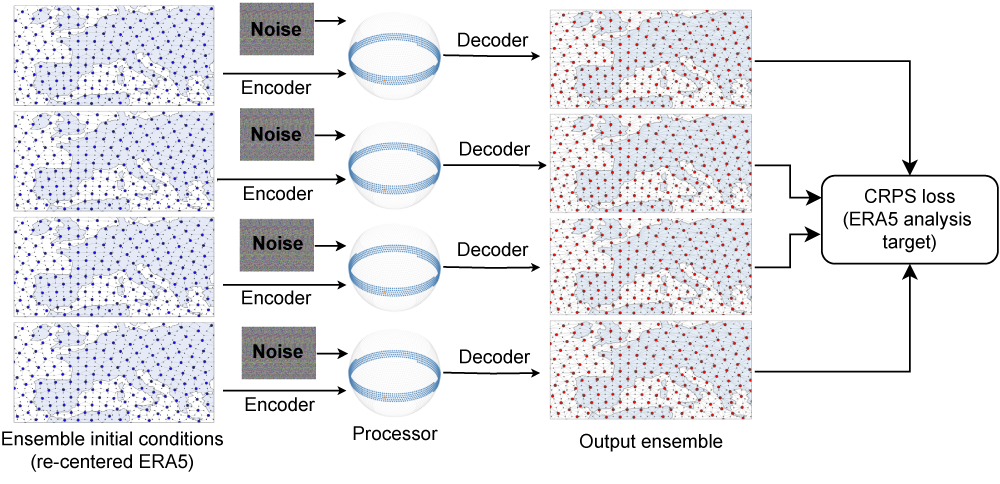
In the AIFS–CRPS configuration, multiple model states (i.e. ensemble members) are propagated forward in time, as shown in Figure 1 (see for example Kochkov et al., 2024). For each ensemble member, a different realisation of random Gaussian noise is injected into the transformer processor. White noise is fed into the model, during both training and inference (forecasting), to be used by AIFS–CRPS to learn a representation of forecast model uncertainty. The CRPS training objective is calculated against the ERA5 deterministic reanalysis at the forecast target time. Perturbed initial conditions are generated by re-centring the ERA5 Ensemble of Data Assimilations (EDA) on the ERA5 deterministic reanalysis. This is consistent with the use of the EDA for ECMWF’s Integrated Forecasting System (IFS), as described in Lang et al., 2015. In addition to model parallelism (sharding, see Lang et al., 2024(a)), the AIFS code can distribute ensemble members across several graphics processing units (GPUs) to enable the training of larger ensembles at higher spatial resolution. AIFS–CRPS also implements autoregressive rollout during training, with 6‑hour time steps; this makes it possible to optimise CRPS up to several days into the forecast. We found that a four-member ensemble was sufficient during training to arrive at a model that shows good probabilistic skill in both training and inference. Larger ensemble sizes are used during inference.

**FIGURE 1** Probabilistic training with CRPS optimisation (AIFS–CRPS): the AIFS propagates four ensemble members that are then optimised jointly through the CRPS loss. The ensemble members can reside on separate GPU devices; in this case, a differentiable all‑gather operation happens before the loss computation. Ensemble member trajectories start from different initial conditions (re-centered ERA5 EDA, see text) and receive different noise inputs.

Diffusion-based training

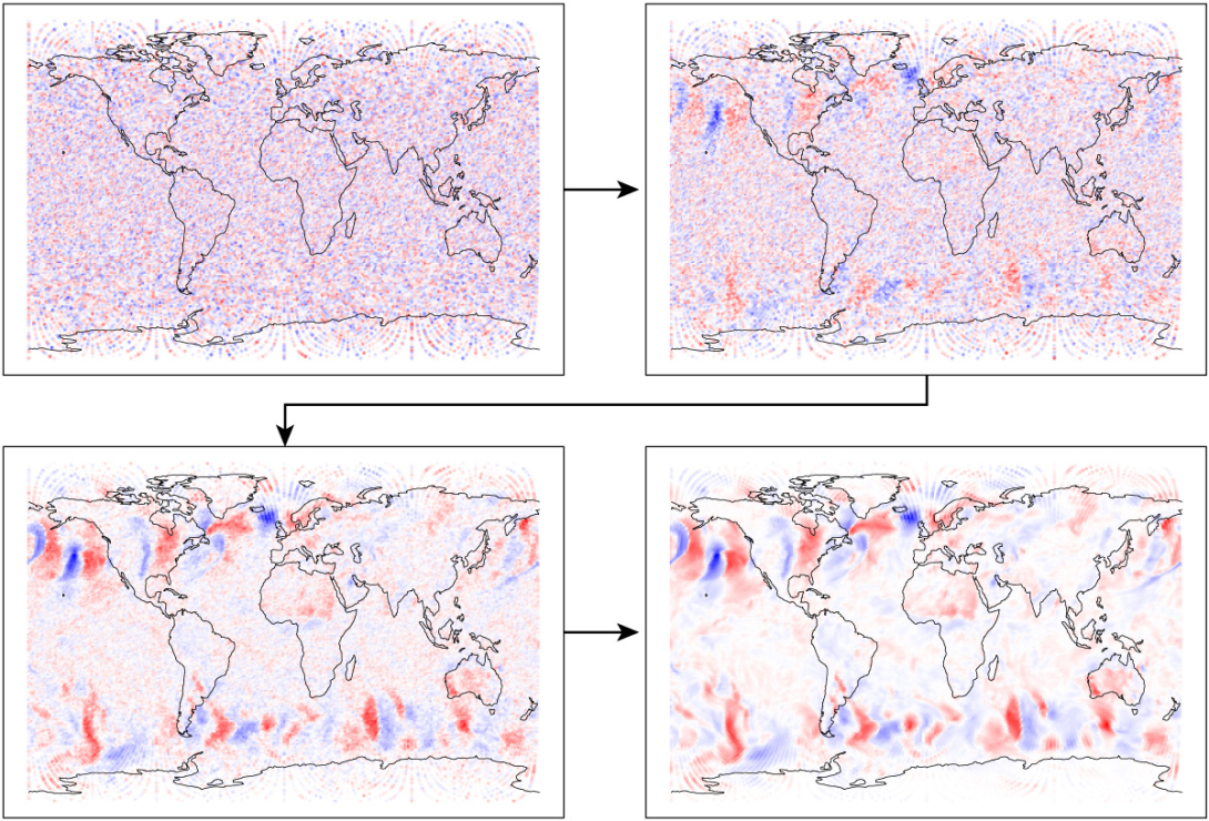
In the diffusion approach (AIFS–Diffusion), the AIFS learns to remove noise from a forecast state, conditioned on the initial conditions and a noise schedule (Price et al., 2024; Karras et al., 2022; and Figure 2). During training, the model ‘sees’ different noise levels, i.e. increasingly noisy forecast states, all the way up to ‘pure’ noise. The model iterates on the same state using a sampling process, arriving at a 12‑hour forecast tendency after 20 denoising steps. This increases the computational cost of a single forecast trajectory. Diffusion-based training usually requires a significantly larger number of training steps than deterministic training. On the other hand, AIFS–Diffusion does not incur the overhead of propagating multiple ensemble members as in AIFS–CRPS. We have found that both ensemble configurations have comparable training costs at a horizontal grid spacing of approximately one degree (111 km).

**FIGURE 2** Diffusion training (AIFS–Diffusion): we show four (non-consecutive) steps from a denoising diffusion chain. Starting from pure Gaussian noise (top left), the model generates a 12-hour tendency (bottom right). The model has many variables and levels; for illustration purposes, the meridional wind component at 850 hPa has been selected.

Inference

During inference, AIFS–CRPS and AIFS–Diffusion start from the initial conditions of the operational IFS ensemble. The initial conditions include the singular vector component of the initial perturbations. Both AIFS–CRPS and AIFS–Diffusion are then run autoregressively to generate 15-day forecasts. The ensembles are configured with a forecast step of 12 hours (AIFS–Diffusion, cf. Price et al., 2024) and 6 hours (AIFS–CRPS). Each ensemble member is independent, and thus the forecast generation is fully parallel. The cost of an AIFS–Diffusion forecast is significantly higher than that of an AIFS–CRPS forecast because the diffusion model is called multiple times per forecast step. That said, both data-driven approaches are very cheap when compared to the computational cost of an IFS ensemble member trajectory: e.g., when run on a single NVIDIA A100 GPU device, AIFS–Diffusion needs only about 2.5 minutes to produce a 15‑day forecast ensemble member. For reference, one IFS Cycle 48r1 ensemble member takes about one hour to produce (excluding I/O), on 96 AMD Epyc Rome central processing units (CPUs). The operational IFS ensemble runs at a spatial resolution of approximately 9 km (Lang et al., 2023).

Forecast evaluation

To enable rapid testing at a small computational cost, we have thus far only trained models at a horizontal grid spacing of one degree, which is consistent with the configuration used for the development of the first deterministic (v0.1) AIFS system.

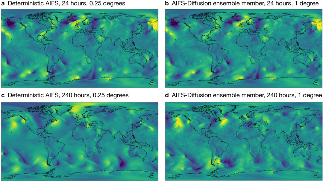
We found that both approaches produce skilful ensemble forecasts. In Figure 3 we compare AIFS–Diffusion and AIFS–CRPS initialised from perturbed, re-centred ERA5 analyses at O96 horizontal grid spacing (ca. one degree) to the 2019 IFS operational ensemble (ca. 18 km horizontal grid spacing). AIFS–Diffusion and AIFS–CRPS produce well-calibrated forecasts and generate realistic forecast variability. In contrast to deterministic AIFS forecasts, probabilistically trained AIFS ensemble members retain a similar level of detail at short- and medium-range lead times, as evidenced in Figure 4.

**FIGURE 3** Fair CRPS scores of (a) 500 hPa geopotential height and (b) 850 hPa temperature, comparing the 50-member operational IFS ensemble with 8-member ensembles initialised from the ERA5 EDA for a 3-month period in 2019, using models trained with the proper score optimisation (AIFS–CRPS) and diffusion (AIFS–Diffusion) techniques.

**FIGURE 4** Depicted are (a) a 24-hour forecast of the deterministically (MSE) trained AIFS at N320 (a forecast with a horizontal grid spacing of ca. 0.25 degrees), (b) a 24-hour AIFS–Diffusion ensemble member at O96 (a forecast with a horizontal grid spacing of ca.1 degree), (c) the same as (a) but showing a 240 h forecast, and (d) the same as (b) but showing a 240 h forecast. The forecasts the AIFS produces after probabilistic training (diffusion or fair CRPS) show a similar level of detail at short- and medium-range lead times.

Implementation

AIFS–Diffusion was chosen as the first candidate for experimental real-time implementation. The operational IFS ensemble provides perturbed initial conditions for the data-driven ensemble forecast. After fine-tuning on operational IFS analyses, the resulting model is competitive with the 9 km IFS ensemble for upper-air scores (see Figure 3 in Lang et al., 2024(b)). It now runs twice daily in a 51‑member configuration and produces a similar set of variables to that of the deterministic AIFS (Lang et al., 2024(b)). It is important to note that, while the control member of the AIFS–Diffusion ensemble configuration is started from unperturbed initial conditions, it nonetheless includes a representation of model uncertainty because of the stochastic sampling involved in calculating the forecast.

To better quantify and understand its forecast performance, the real-time AIFS–Diffusion ensemble is periodically evaluated by ECMWF analysts – see, e.g., the recent episode of exceptionally heavy rainfall in the United Arab Emirates described by Magnusson et al., 2024.

A cold snap over western Europe

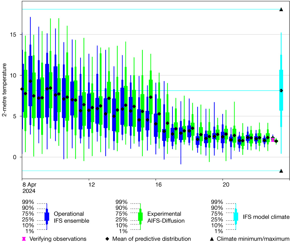
The forecasting skill of the diffusion-trained ensemble can be illustrated with an example from France. A cold spell was observed over parts of central and western Europe in late April 2024. The cold air caused late-season, potentially damaging frost during the flowering period of fruit trees and grapevines. Figure 5 shows 2‑metre temperature ensemble forecasts from the IFS ensemble and the experimental real-time AIFS–Diffusion ensemble. The forecasts are averaged over a 1x1-degree box located near Troyes, France, a winemaking region. Both forecasting systems successfully forecast the 24 April cold anomaly about 8–10 days before the event.

**FIGURE 5** Ensemble forecasts of 2-metre temperature ahead of a cold spell over Europe, in late April 2024. The forecasts are averaged over a 1x1-degree box centred around 48.3°N, 4°E (near Troyes, France).

Sub-seasonal forecasts

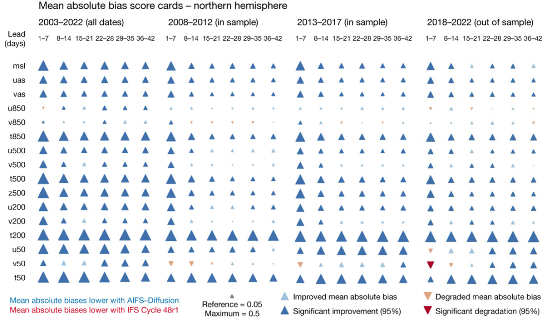
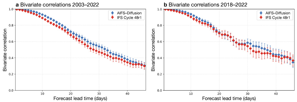
Early evidence strongly suggests that the ensemble AIFS will also have a role to play in sub-seasonal forecasting. While deterministically trained data-driven forecast models are known to develop large biases over relatively long forecast horizons (Ben‑Bouallègue et al., 2023), the systematic errors of the two probabilistic models described here are comparable to or smaller than the biases of the physics-based IFS, for a range of forecast parameters (see Figure 6 for AIFS–Diffusion vs the IFS). Notably, preliminary analyses of sub-seasonal AIFS–Diffusion ensembles show significant forecast skill, outperforming (weeks 1 and 2) or matching (week 3 and later) the skill of the IFS when predicting the Madden–Julian Oscillation (MJO), as shown in Figure 7.

**FIGURE 6** Scorecard summarising changes in mean absolute bias (MAB) for the northern hemisphere (30°N–90°N) for AIFS–Diffusion versus operational IFS (Cycle 48r1) sub-seasonal hindcasts, calculated as 1 – MAB_AIFS/MAB_IFS as described in Roberts et al. (2021). MAB is shown estimated for all available dates (2003–2022; left) and three different 5-year subsets, including data not used for training (2018–2022; right). Upward (blue) triangles indicate that absolute biases aggregated across all locations and start dates in AIFS–Diffusion are reduced compared to IFS Cycle 48r1. The variables shown are mean sea-level pressure (msl) and zonal/meridional wind at 10 m (uas/vas); temperature (t) and zonal/meridional wind (u/v) at different pressure levels (850, 500, 200 and 50 hPa); and geopotential height (z) at 500 hPa. For both systems, MAB is calculated relative to ERA5 using 8-member 46-day ensemble forecasts initialised every Monday and Thursday within the re-forecast period. Symbol areas are proportional to the fractional change in bias score and significance from the distribution created by block-bootstrap resampling of the available start dates.

**FIGURE 7** Bivariate correlations for an MJO index calculated from 200 hPa and 850 hPa zonal wind anomalies for AIFS–Diffusion (blue) and IFS Cycle 48r1 (red) calculated (a) using all available dates (2003–2022) and (b) data not used for training (2018–2022). Higher correlations mean better forecasts. The MJO index used here is an approximation for the full Wheeler and Hendon (2004) Real-time Multivariate MJO index as it excludes contributions from outgoing longwave radiation that are not available from AIFS–Diffusion. For both systems, correlations are calculated relative to ERA5 using 8-member 46-day ensemble forecasts initialised every Monday and Thursday within the re-forecast period. Error bars represent the 2.5th and 97.5th percentiles of the distribution created by block-bootstrap resampling of the available start dates.

Outlook

Probabilistic training of data-driven models results in skilful ensemble forecasts that also overcome one of the main limitations of deterministically trained models: the over-smoothing of forecast fields. Ongoing research aims to further increase forecast skill, to improve the fine-tuning approaches of the ensemble models on operational IFS analyses, to increase the temporal resolution, and to decrease horizontal grid spacing to 0.25 degrees. It is likely that higher-resolution ensembles will improve forecast scores for surface fields such as 2‑metre temperature, precipitation, and 10‑metre winds, as well as the representation of tropical cyclones.

Because data-driven ensemble forecasts are much cheaper to produce than their physics-based counterparts, it will be possible to add an AIFS–CRPS ensemble configuration to the experimental real-time suite, running alongside the diffusion-based system. This will allow a comprehensive evaluation of the strengths and weaknesses of both approaches.

Meteograms along with mean and spread products from the experimental AIFS real-time ensemble are available as open charts (https://charts.ecmwf.int) under ECMWF’s open data policy. Further charts and data will be available in the near future.

Editorial

News

Earth system science

Newsletter