Ensemble forecasts need to account for uncertainties in both initial conditions and the forecast model. Since 1998, the latter uncertainties have been represented in ECMWF’s Integrated Forecasting System (IFS) via the Stochastically Perturbed Parametrization Tendency scheme (SPPT; Buizza et al., 1999). This scheme is also referred to as ‘stochastic physics’. It has been revised several times. SPPT has played an important role through increasing the ensemble spread and boosting the probabilistic skill of ECMWF ensemble forecasts over the past 25 years (see Lock et al., 2019, for details of the operational SPPT configuration). In IFS Cycle 49r1, which will be implemented in November 2024, SPPT will be replaced by the Stochastically Perturbed Parametrizations (SPP) scheme in all ensemble applications. SPP has been developed over several years (Ollinaho et al., 2017; Lang et al., 2021). It represents model uncertainties closer to the sources of errors. The remainder of the article explains the motivation for this revision and how the new scheme works, and it sets out the impacts expected from the revision of the model uncertainty representation.
Motivation
While SPPT has been a success story in terms of its impact on the skill of ensemble forecasts, awareness of some drawbacks has increased over the years. This fuelled interest in developing a representation of uncertainties that has a comparable positive impact on ensemble skill to SPPT, but which can bring additional benefits. In particular, we seek a perturbation method that maintains the conservation properties of the unperturbed model, by ensuring that fluxes at the surface and top of the atmosphere respond consistently to the perturbations within the atmospheric column. Furthermore, by applying the perturbations to individual physical processes, we can introduce a representation of errors in, for example, the shape of a heating profile, and remove the need to taper perturbations near the surface.
Methodology
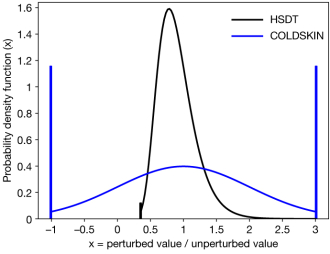
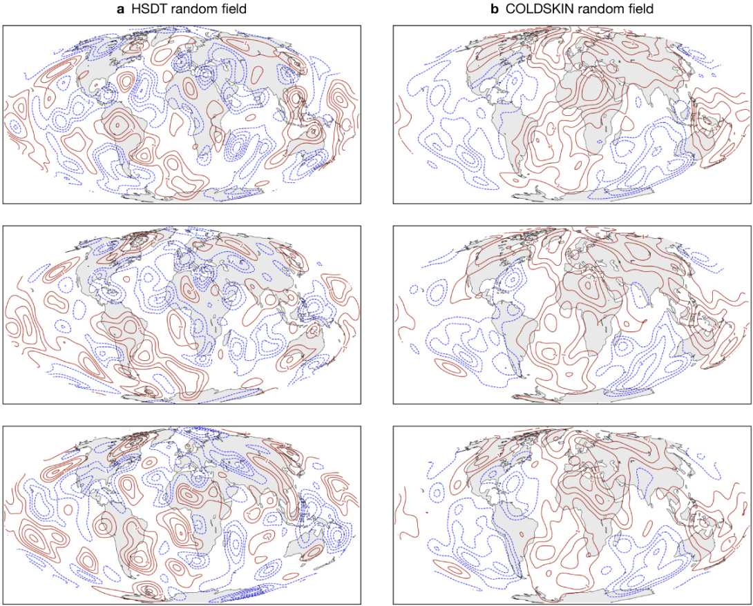
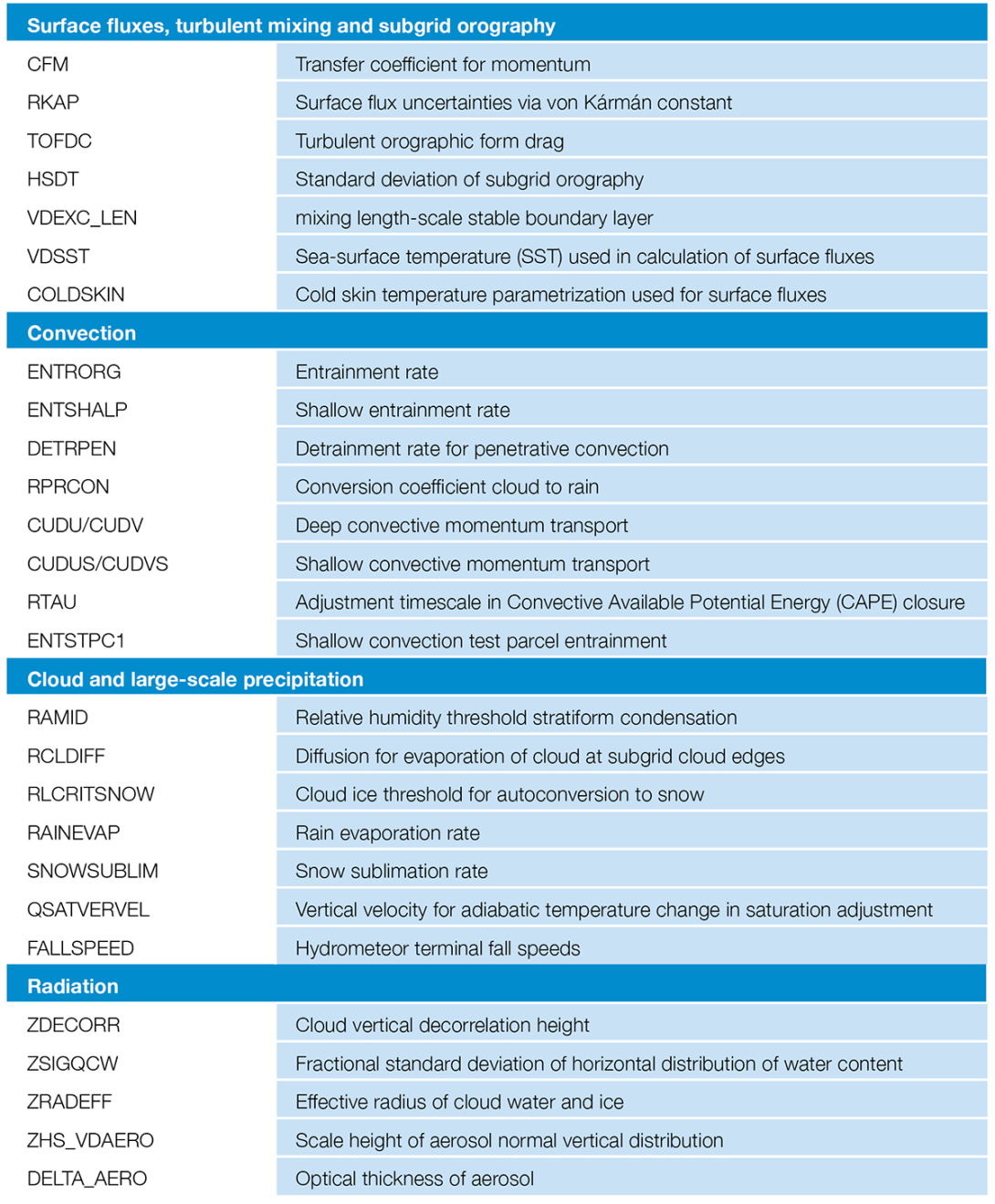
SPP is a stochastic representation of uncertainties which targets uncertain elements within the parametrizations of individual physical processes. The elements are identified by scientists who develop the parametrizations and have in-depth knowledge of the sensitivities of their schemes to specific choices that need to be made to constrain the parametrization. The version of SPP in Cycle 49r1 has 27 perturbed elements in order to represent the dominating uncertainties in the parametrizations of convection, large-scale cloud, radiation, surface exchanges, vertical turbulent mixing, and orographic gravity wave drag (Table 1). Each perturbation element has its own probability distribution, which is anchored to the unperturbed values used in the deterministic model. Figure 1 shows the distributions sampled by SPP for the elements perturbing the standard deviation of the subgrid orography (HSDT) and the ocean cold skin temperature parametrization (COLDSKIN). The distributions of these elements are limited to a finite range to ensure numerical stability. The distributions are sampled via evolving random fields with prescribed time and space scales (see Lang et al., 2021, for details). Each perturbation element has its own independent random field. Figure 2 displays the evolution of the HSDT and COLDSKIN random fields over three days for one ensemble member. The gridpoint values of the random fields are transformed such that they sample the specified probability distributions. The random fields have two components with spatial decorrelation scales of 1,000 km and 3,000 km and corresponding decorrelation time scales of 3 days and 30 days, respectively. The development of the scheme required a number of iterations to constrain the distributions of all elements in order to generate the right level of variance in ensembles at all lead times, using one unified configuration.
SPP inherits the local conservation properties from the deterministic parametrizations. The fluxes at the surface and at the top of the atmosphere are computed using the perturbed elements, resulting in perturbed fluxes that remain consistent with the tendencies in the atmospheric column. Due to the use of multiple perturbation elements, the structure of the tendencies can be altered by the perturbations and can represent, for instance, uncertainties in the shape of heating profiles.
Impacts
Now, we provide an overview of the impacts of SPP on local conservation and on the different ranges of ECMWF’s forecasts, from the medium range (up to 15 days) via the sub-seasonal range (up to 46 days) to the seasonal range (up to 13 months), as well as in km‑scale ensemble forecasts explored in the EU’s Destination Earth (DestinE) initiative.
Local conservation
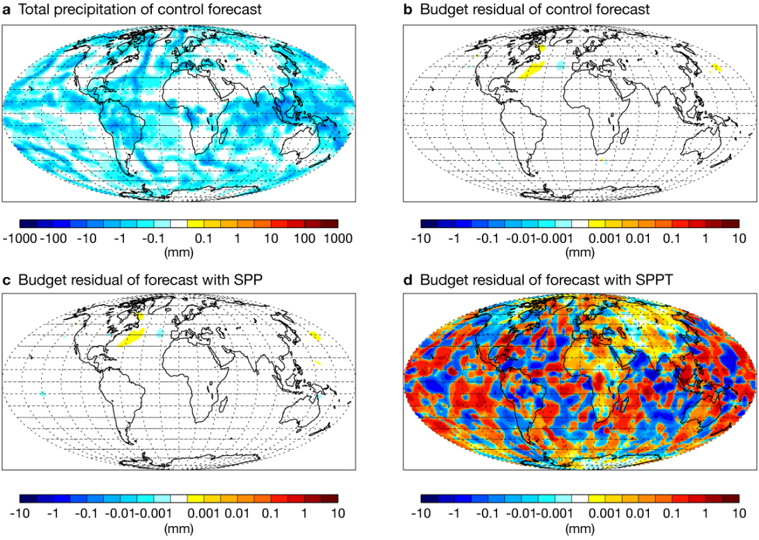
The parametrizations of physical processes aim to conserve moisture and enthalpy (moist static energy). Column integrals of the tendencies together with the fluxes at the surface and the top of the atmosphere form a nearly closed budget when the semi-Lagrangian averaging of the physics tendencies is deactivated (see Part IV of the IFS documentation for details: https://www.ecmwf.int/en/publications/ifs-documentation). Figure 3 (a,b) shows that the residual term in the budget for moisture is very small compared to the precipitation flux in the unperturbed control forecast. The forecast perturbed with SPP achieves a similar level of conservation as the control forecast, while the forecast perturbed with SPPT has a residual that is locally nearly of the same magnitude as the precipitation flux itself (Figure 3 c,d). The level of conservation or lack of conservation shown in the figure for forecast lead times of 45 to 48 hours is representative for all forecast lead times, and it is also representative for other ensemble members or start dates.
For the local budget of enthalpy, the level of conservation of forecasts perturbed with SPP is again similar to the level of conservation in the unperturbed control forecast, while the forecasts using SPPT show large residuals.
Medium-range forecasts
Tropospheric scores in the extratropics are overall improved with SPP, e.g. geopotential (see Figure 4a). Upper-air scores in the tropics are more mixed, with improvements at some levels and degradations at others. For example, there is a strong positive impact for temperature in the tropics at 500 hPa and 250 hPa. Here, SPP shows improvements of around 10%.
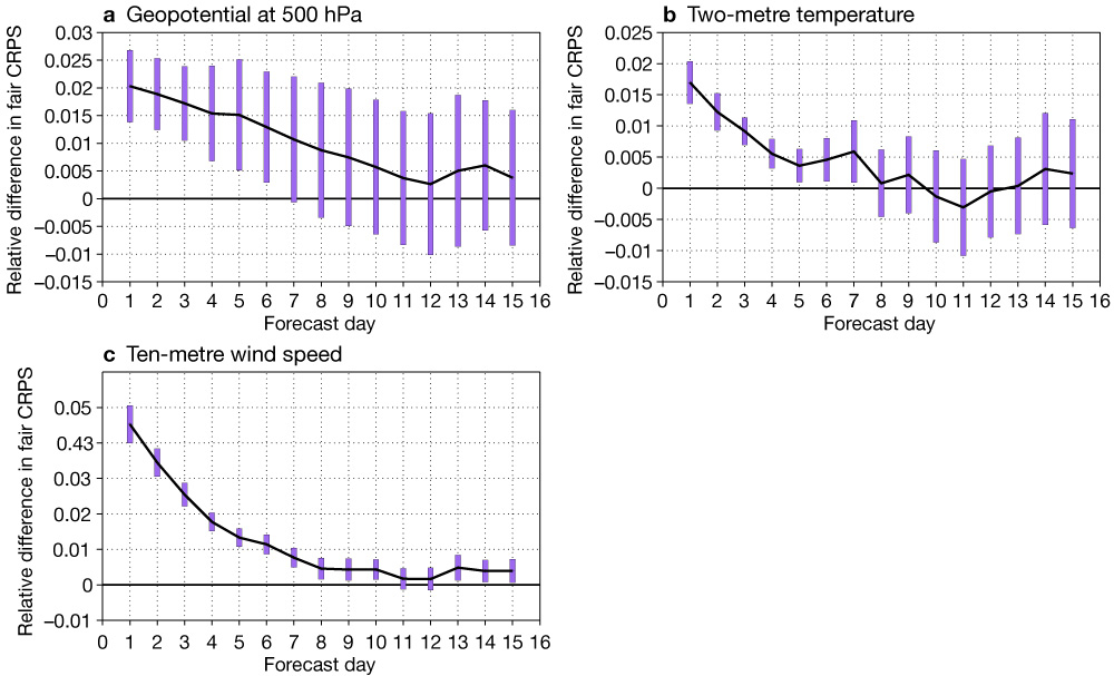
Conversely, wind scores in the tropics are degraded, between 1 and 2% for some levels. In general, upper-air spread (ensemble standard deviation) is somewhat decreased, around 1 to 2% in the extratropics. Forecast skill of surface variables like 2-metre temperature and 10-metre wind speed is improved (Figure 4b and c). While 2‑metre temperature spread is quite similar, spread of 10‑metre wind is increased, by around 25% at a lead time of 48 hours.
SPP results in a noticeable increase in the occurrence frequency of tropical cyclones in the ensemble. The impact on tropical cyclone frequencies originates mainly from the SPP perturbations in the convection parametrization, specifically the perturbations to the deep convective momentum transport (CUDUDV). We have compared the occurrence frequencies to tropical cyclone data from the international best track archive for climate stewardship (IBTrACS). For wind speeds exceeding 20 m/s, the increase in tropical cyclone frequency appears to bring the forecasts closer to the observed frequencies. We believe that for weaker systems, with wind speeds less than 20 m/s, the observed frequencies in IBTraCS may be underestimated.
Sub-seasonal forecasts
In broad terms, the response in sub-seasonal forecasts to changing from SPPT to SPP is similar to that in the medium range. There are small changes in spread (typically of a few percent) throughout forecast lead times. The changes are characterised by reduced spread in upper‑air fields and increased spread in surface fields. They are most pronounced in the tropics. The reduced spread with SPP tends to translate into improved spread–error ratios, since using SPPT in the latest ensemble configuration generates somewhat over-dispersive forecasts of some upper‑air fields.
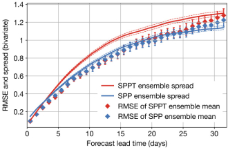
A key component of predictability in longer-range forecasts derives from the Madden–Julian Oscillation (MJO, see e.g. Lin et al., 2009). The MJO is a large-scale weather pattern that occurs over the Indian and Pacific Oceans and is associated with global teleconnection patterns. Figure 5 illustrates ensemble spread and root-mean-square error (RMSE) of the ensemble mean for the real-time multivariate MJO (RMM) index (following Wheeler and Hendon, 2004) from two sets of re‑forecasts: one using SPPT and one SPP. The RMM index is constructed from a combination of tropical upper-air fields: zonal (east–west) winds at 850 hPa and 200 hPa, and outgoing longwave radiation. The goal is a good match between ensemble spread and RMSE. While the forecast skill (represented by the RMSE of the ensemble mean) for the two model uncertainty representations remains very similar, the ensemble spread with SPP is significantly reduced from that with SPPT, and it matches the error much more closely.
Seasonal forecasts
Although the change from SPPT to SPP will not be applied to operational seasonal forecasts until the next upgrade of the seasonal system (to SEAS6), the impact of the change has been tested in seasonal configurations.
Switching from SPPT to SPP tends to reduce ensemble spread. For some key forecast variables, that reduction in spread addresses an over-dispersive signal from SPPT. This translates into improved spread–error ratios. For example, for equatorial Pacific regions that are important for El Niño–Southern Oscillation (ENSO) predictions, the spread–error ratios for sea-surface temperatures (SSTs) are mostly improved by the reduced spread with SPP.
The change of the model uncertainty scheme also impacts some forecast biases over these longer lead times. For example, for SSTs in the eastern equatorial Pacific, SPP leads to some warming, while SPPT tends to cool the region. The consequence of the bias changes is complicated, since for both schemes there are regions and seasons for which the change helps (or hinders) by counteracting (or strengthening) the prevailing forecast bias. However, the differences are small relative to the underlying biases.
Kilometre-scale ensemble forecasts
Replacing SPPT with SPP brings benefits in km-scale ensemble forecasts (at a grid spacing of 4.4 km) similar to those in the medium-range. In the tropics, fair CRPS scores for wind speed are slightly degraded for 500 and 850 hPa levels, and for temperature at 850 hPa.
However, surface fair CRPS scores (evaluated against observations) improve between 2 and 5% for 2‑metre temperature and 10‑metre wind speed. For several extreme weather events (e.g. tropical cyclones, extreme precipitation) evaluated with the km‑scale ensemble explored within the EU’s Destination Earth (DestinE) initiative, the SPP scheme seems to generally provide better probabilistic predictions and introduces more ensemble spread than SPPT. Furthermore, forecasts using SPP have 24‑hour precipitation distributions over the tropics that better match observations (based on IMERG satellite precipitation) than those produced with SPPT.
Conclusion and outlook
Adopting SPP restores the physical consistency of the ensemble members to the level of the unperturbed forecast. With SPP, precipitation, evaporation, sensible and latent heat fluxes as well as perturbed radiative fluxes are consistent with the perturbations in the atmospheric column. This leads to a degree of local conservation of moisture and enthalpy comparable to that achieved in the unperturbed forecast. With SPPT, the forecasts exhibit residuals which are on average at least an order of magnitude larger than the residuals in the control forecast. Moreover, the combination of many independent perturbed elements across the different parametrizations permits introducing a representation of uncertainties that goes beyond amplitude errors of the total physics tendencies. It permits, for instance, the representation of uncertainties in the shape of a heating profile.
The replacement of SPPT with SPP in Cycle 49r1 is the result of a major complex development effort, which had to balance requirements across lead times of hours in the Ensemble of Data Assimilations (EDA) to months in seasonal forecasts. Both SPPT and SPP have some effect on mean errors. The bias changes with SPPT can compensate the mean errors of the unperturbed model for some variables and regions of the atmosphere. In general, the mean errors of forecasts perturbed with SPP are closer to the mean errors of the unperturbed forecast than when SPPT is used. This is a desirable feature that will support IFS development in the future. However, it has the inevitable effect that biases increase for some variables and some regions when SPP replaces SPPT.
Noticeable improvements in skill with the introduction of SPP are achieved for 2‑metre temperature and 10‑metre wind. Further improvements will appear via the use of SPP in the EDA in Cycle 49r1. SPP has helped to address the underdispersion in the boundary layer, which has been seen as a limiting factor for the assimilation of 2‑metre temperature observations. The introduction of SPP together with other changes in the EDA (higher resolution and soft re-centring) has permitted reducing the amplitude of the singular vector initial perturbations. This will partly address the overdispersion in the winter storm tracks in the early medium range.
In the coming years, it is planned to extend SPP into the parametrizations of the land surface. An initial investigation has explored the beneficial impact of increased ensemble spread from stochastic perturbations to land surface parameters in the context of land data assimilation.
SPP has gained popularity as a representation of model uncertainties and has been introduced already in the Canadian Global Ensemble Prediction system and in the regional HARMONIE ensemble prediction system (McTaggart-Cowan et al., 2022; Tsiringakis et al., 2024).
Further reading
Buizza, R., M. Miller & T.N. Palmer, 1999: Stochastic representation of model uncertainties in the ECMWF ensemble prediction system. Q. J. R. Meteorol. Soc., 125, 2887–2908.
Lang, S.T., S.-J. Lock, M. Leutbecher, P. Bechtold & R.M. Forbes, 2021: Revision of the Stochastically Perturbed Parametrisations model uncertainty scheme in the Integrated Forecasting System. Q. J. R. Meteorol. Soc., 147, 1364–1381.
Lin, H., G. Brunet & J. Derome, 2009: An Observed Connection between the North Atlantic Oscillation and the Madden–Julian Oscillation. J. Climate, 22, 364–380.
Lock, S.-J., S.T.K. Lang, M. Leutbecher, R.J. Hogan & F. Vitart, 2019: Treatment of model uncertainty from radiation by the Stochastically Perturbed Parametrization Tendencies (SPPT) scheme and associated revisions in the ECMWF ensembles. Q. J. R. Meteorol. Soc., 145, 75–89.
McTaggart-Cowan, R., L. Separovic, R. Aider, M. Charron, M. Desgagné, P.L. Houtekamer et al., 2022: Using stochastically perturbed parameterizations to represent model uncertainty. Part I: Implementation and parameter sensitivity. Mon. Wea. Rev., 150, 2829–2858.
Ollinaho, P., S.-J. Lock, M. Leutbecher, P. Bechtold, A. Beljaars, A. Bozzo et al., 2017: Towards process‐level representation of model uncertainties: Stochastically Perturbed Parametrizations in the ECMWF ensemble. Q. J. R. Meteorol. Soc., 143, 408–422.
Tsiringakis, A., I.-L. Frogner, W. de Rooy, U. Andrae, A. Hally, S. Contreras Osorio et al., 2024: An Update to the Stochastically Perturbed Parametrizations Scheme of HarmonEPS. Mon. Wea. Rev., 152, 1923–1943. https://doi.org/10.1175/MWR-D-23-0212.1
Wheeler, M. C. & H.H. Hendon, 2004: An All-Season RealTime Multivariate MJO Index: Development of an Index for Monitoring and Prediction. Mon. Wea. Rev., 132, 1917–1932.
